Building the Map

In Section 3.1 we mentioned that when the robot has four landmarks in its viewframe, it creates a new beta-unit for them. However, with four landmarks, there are four candidates to be the target of the beta-unit. Moreover, if the robot has more than four landmarks in the viewframe, there are many possible beta-units to be created. More precisely, if there are $n$ visible landmarks, there are ${n \choose 4} \cdot 4$ candidates for being new beta-units. However, it is not feasible to store them all, firstly because of the huge number of combinations, and secondly, and more important, because some configurations are better than others. Thus, some selection criterion must be used.

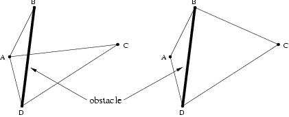
Before describing the criterion we have used, we explain how the obstacles are represented in the map. We differentiate two types of obstacles: point obstacles and linear obstacles. Point obstacles are those the robot can easily avoid by slightly modifying its trajectory, since they do not completely block the path. In our indoor environment such obstacles are boxes and bricks. In outdoor environments they could be small rocks, trees, etc. These obstacles do not affect the global navigation, as the Pilot can tackle them alone, so the Navigation system does not take them into account and they are not stored in the map. On the other hand, linear obstacles are long obstacles that completely block the path of the robot. They can also be avoided by the Pilot, but the trajectory has to be drastically modified. In our indoor environment we use several bricks to form these obstacles. In an outdoor environment these obstacles could be fences, walls, groups of rocks, etc. Since these obstacles do highly affect the navigation task, they have to be represented in the map, so that they are taken into account when computing routes to the target. The information about these obstacles is stored on the arcs of the topological map. An arc is labelled with an infinite cost to indicate that there is an obstacle between the two regions connected by the arc. Notice that with this representation we can only represent those obstacles placed along the line connecting two landmarks. Although in our experiments we have designed the environments so that they satisfy this condition, the system would also work if it were not satisfied. However, in this latter case, the Navigation system could not take all the obstacles into account, and thus, its performance would be worse. The arcs' labels are updated whenever the Pilot system informs about the presence of an obstacle between two landmarks.

Going back to the selection criterion, given a set of landmarks, for which their location is known, we seek to obtain a set of triangular regions with the following constraints:

• Low collinearity: the collinearity of a region is computed as
  

  $$Col(R) = 1 - \frac{\alpha \beta \gamma}{(\frac{\pi}{3})^3}$$ (4)

  
  
  where $\alpha$, $\beta$ and $\gamma$ are the three angles of the triangular region. The best quality is associated to equilater triangles, where $\alpha=\beta=\gamma=\frac{\pi}{3}$, and hence their collinearity is 0. When one of the angles is 0, landmarks would be maximally collinear and $Col(R)=1$. The higher the collinearity, the higher the error on the computation of the $\beta$-vector and landmark locations (see [55] for a detailed explanation). Therefore, the regions with lower collinearity are preferred. For example, in Figure 3.4 the two regions on the right are preferred over the two on the left, since the region ABD is too collinear.

  Figure 3.4: Left: bad set of regions; region ABD is too collinear. Right: good set of regions

  

• Connectivity: the set of regions must be converted into a graph with a single component, so that there is a path between any two nodes of the graph. In Figure 3.5, the set of regions on the left is not acceptable, since there are two disconnected components, whereas in the set on the right all the regions are connected.

  Figure 3.5: Left: bad set of regions; there are two disconnected components. Right: good set of regions

  

• Convex hull covering: the regions must cover the convex hull of the set of landmarks, so that the environment is represented completely, with no unrepresented regions. In Figure 3.6, the set on the left is not acceptable, since the region DFG is not represented.

  Figure 3.6: Left: bad set of regions; region DFG is missing. Right: good set of regions

  

• Non overlapping: the regions should not overlap with each other. If this were the case, the robot could be in more than one region at the same time, which could cause some problems when computing routes to the target. For instance, if the robot were in the overlapping area of the two regions, it would make no sense to order the robot to move from one region to the other, since it would already be inside both regions, and the order would not have any effect. Moreover, if one of the overlapping edges is an obstacle, the path from one side of the adjacent region to the other side would be blocked, which is obviously a bad representation of the environment, since the robot must be able to move around the whole space of a region. In Figure 3.7, the set of regions on the left is a bad set, since part of the obstacle between landmarks B and D lies inside the region ADC. In this case, the associated graph would have two nodes, ABD and ACD, which would be connected, so the robot would think that it can move from region ABD to region ADC, but it would find the path blocked because of the obstacle.

  Figure 3.7: Left: bad set of regions; the obstacle between landmarks B and D is inside the region ACD. Right: good set of regions

  

• Keep obstacles: if an edge of a region is marked as an obstacle, this edge must be kept in the map, even if it causes the robot to keep high collinear regions. The obstacle edges are the only ones that cannot be removed from the map. If we did so, the information about the location of obstacles would be lost and would not be taken into account when computing routes to the target.

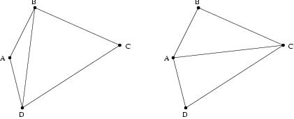
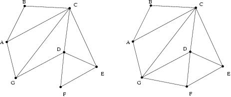
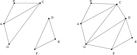
To compute the optimal set of regions for a given set of landmarks, we have developed an incremental algorithm that treats landmarks one by one to update the map. However, the algorithm only starts working when the locations of at least four landmarks are known, since this is the number of landmarks needed to create a beta-unit. With these four landmarks, the mapping algorithm computes the best set of regions according to the constraints given above. Then, the rest of visible landmarks, if any, are added one by one to the already built map. When adding a new landmark to the map, two situations can happen: (1) the landmark is inside an already existing region, or (2) the landmark is outside any region. In the first case, the region containing the new landmark is replaced by three new regions (see Figure 3.8). In the second case, all the possible new regions are created (see Figure 3.9). No matter the situation of the landmark, once the new regions have been created, the algorithm checks if the resulting map is still optimal. This optimization consists of analyzing each pair of adjacent regions and checking if their configuration is optimal according to the constraints. If it finds that some regions could be changed so that a better configuration is obtained, it does so. An example of this step by step updating is shown in Figure 3.10.

Figure 3.8: Adding a new landmark (D) located inside an existing region (ABC) resulting in the substitution of the original region for three new regions (ABD,ACD,BCD)

Figure 3.9: Adding a new landmark (D) located outside any existing region resulting in the addition of two new regions (ACD,BCD)

Figure 3.10: Adding a new landmark (E) into a map with two regions (ABD and BCD): first, region ABD is substituted for three new regions (ABE,ADE,BDE); after that, optimization for regions BCD and BDE is performed and they are substituted for the new regions BCE and CDE

Once the set of regions is computed, new beta and topological units can be created. For each new region a beta-unit is created for each region adjacent to it, taking the three landmarks of the first region as the encoding landmarks, and the landmark of the second region that is not in the first one as the target. In other words, for each pair of adjacent regions, two ``twin'' beta-units are created. An example can clarify this explanation: with the regions ABC and ACD shown on the right in Figure 3.4, the beta-units ABC/D and ACD/B would be created. One topological unit is also created for each new region, and the graph is updated according to the adjacency of regions. Initially, the arcs are labelled with a default cost of 1, and they are changed to $\infty$ whenever an obstacle is detected. The topological units corresponding to regions that are not used any more are removed from the graph. However, beta-units are never removed, since they add robustness to the system, as in Section 3.1.

This triangulation algorithm needs the location of the landmarks to be known (either recognized by the Vision system or computed by the beta-coefficient system). However, not all landmark locations can always be known. The algorithm only takes into account those landmarks whose locations are known. This ensures that the five constraints explained above are satisfied only for the located landmarks. When one of the unlocated landmarks is seen or computed, some constraints might become unsatisfied. Whenever any constraint is broken, the map is rebuilt in order to satisfy again all the constraints. This constraint break can also be caused by the fuzziness of the locations. Because of the imprecision of the locations, the map can suddenly be breaking some of the constraints. To avoid having an inconsistent map, every once in a while the satisfaction of the constraints is checked, and, if needed, the map is rebuilt.