Next: Extending Prescott's System: Moving Up: Mapping and Navigation Previous: Mapping and Navigation
The idea behind Prescott's model is to encode the location of a
landmark (which we refer to as target - not to confuse with the
target or goal of the Navigation system)
with respect to the location of three other landmarks.
Having seen three landmarks and a target
from a viewpoint (e.g., landmarks ![]() ,
, ![]() and
and ![]() and
target
and
target ![]() from viewpoint
from viewpoint ![]() , in Figure 3.1), the
system is able to compute the target's position when seeing
again the three landmarks, but not the target, from another
viewpoint (e.g.,
, in Figure 3.1), the
system is able to compute the target's position when seeing
again the three landmarks, but not the target, from another
viewpoint (e.g., ![]() ). A vector, called the
). A vector, called the ![]() -vector of
landmarks A, B, C and T, is computed as
-vector of
landmarks A, B, C and T, is computed as
| (2) |
It should be noted that, although Prescott's system works with Cartesian coordinates, once all the computations have been done, the resulting target's location is converted to polar coordinates, since, as will be seen in next chapters, this is the coordinate system that uses the Navigation system.
![\includegraphics[height=3cm]{figures/abct}](img30.png) |
This method can be implemented with a two-layered network. Each
layer contains a collection of units, which can be connected to
units of the other layer. The lowest layer units are
object-units, and they represent the landmarks the robot has
seen. Each time the robot recognizes a new landmark, a new
object-unit is created. The units of the highest layer are
beta-units and there is one for each ![]() -vector
computed.
-vector
computed.
When the robot has four landmarks in its viewframe, it
selects one of them to be the target, a new beta-unit is created,
and the ![]() -vector for the landmarks is calculated. This
beta-unit will be connected to the three object-units associated
with the landmarks (as incoming connections) and to the
object-unit associated with the target landmark (as an outgoing
connection). Thus, a beta-unit will always have four connections,
while an object-unit will have as many connections as the number
of beta-units it participates in. An example of the network can be
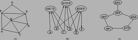
seen in Figure 3.2b. In this figure there are six
object-units and three beta-units. The notation ABC/D is
understood as the beta-unit that computes the location of landmark
D when the locations of landmarks A, B and C are known.
-vector for the landmarks is calculated. This
beta-unit will be connected to the three object-units associated
with the landmarks (as incoming connections) and to the
object-unit associated with the target landmark (as an outgoing
connection). Thus, a beta-unit will always have four connections,
while an object-unit will have as many connections as the number
of beta-units it participates in. An example of the network can be
seen in Figure 3.2b. In this figure there are six
object-units and three beta-units. The notation ABC/D is
understood as the beta-unit that computes the location of landmark
D when the locations of landmarks A, B and C are known.
This network has a propagation system that permits the robot to compute the location
of non-visible landmarks. It works as follows: when the robot
sees a group of landmarks, it activates (sets the value) of the associated
object-units with the egocentric locations of these landmarks. When an
object-unit is activated, it propagates its location to the beta-units
connected to it. On the other hand, when a beta-unit receives the location
of its three incoming object-units, it gets active and
computes the location of the target it encodes using its ![]() -vector,
and propagates the result to the object-unit representing the target. Thus,
an activation of a beta-unit will activate an object-unit that can activate
another beta-unit, and so on. For example, in the network of Figure
3.2b, if landmarks A, B and C are visible, their object-units will
be activated and this will activate the beta-unit ABC/D, computing the location
of D, which will activate BCD/E, activating E, and causing BDE/F also to be
activated. In this case, knowing the location of only three landmarks (A, B and C), the
network has computed the location of three more landmarks that were not
visible (D, E and F).
This propagation system makes the network compute all possible landmarks'
locations. Obviously, if a beta-unit needs the location of a landmark that
is neither in the current view nor activated through other beta-units, it will
not get active.
-vector,
and propagates the result to the object-unit representing the target. Thus,
an activation of a beta-unit will activate an object-unit that can activate
another beta-unit, and so on. For example, in the network of Figure
3.2b, if landmarks A, B and C are visible, their object-units will
be activated and this will activate the beta-unit ABC/D, computing the location
of D, which will activate BCD/E, activating E, and causing BDE/F also to be
activated. In this case, knowing the location of only three landmarks (A, B and C), the
network has computed the location of three more landmarks that were not
visible (D, E and F).
This propagation system makes the network compute all possible landmarks'
locations. Obviously, if a beta-unit needs the location of a landmark that
is neither in the current view nor activated through other beta-units, it will
not get active.
This propagation system adds robustness to the computation of
non-visible landmarks, since a landmark can be the target of several
beta-units at the same time. Because of imprecision in the perception on
landmark locations, the estimates of the location of a target using
different beta-units are not always equal. When this happens, the
different location estimates must be combined. Prescott
uses the size of the ![]() -vector as the criterion
to select one among them. A beta-unit with a smaller
-vector as the criterion
to select one among them. A beta-unit with a smaller
![]() -vector is more precise than those with larger
-vector is more precise than those with larger
![]() -vectors (see [55] for a detailed discussion on how to
compute the estimate error from the size of the
-vectors (see [55] for a detailed discussion on how to
compute the estimate error from the size of the ![]() -vector).
The propagation system does not only propagate location estimates, but
also the size of the largest
-vector).
The propagation system does not only propagate location estimates, but
also the size of the largest ![]() -vector that has been used to
compute each estimate.
When a new location estimate
arrives to an object-unit, its location is substituted with the new
one if the size of the largest
-vector that has been used to
compute each estimate.
When a new location estimate
arrives to an object-unit, its location is substituted with the new
one if the size of the largest ![]() -vector used is smaller than
that used for the last location estimate received.
-vector used is smaller than
that used for the last location estimate received.
The network created by object and beta units can be converted into a graph where the nodes represent triangular shaped regions delimited by a group of three landmarks, and the arcs represent paths. These arcs can have an associated cost, representing how difficult it is to move from one region to another. Although the arcs are created immediately when adding a new node to the graph, the costs can only be assigned after the robot has moved (or tried to move) along the path connecting the two regions. In the case the path is blocked by an obstacle, the arc is assigned an infinite cost, representing that it is not possible to go from one region to the other. This graph is a topological map, and we call its nodes topological units. An example of how the topology is encoded in a graph is shown in Figure 3.2c.
 |
This topological map is used when planning routes to the target. Sometimes, when the position of the target is known, the easiest thing to do is to move in a straight line towards it, but sometimes it is not (the route can be blocked, the cost too high...). With the topological map, a route to the target can be computed. In Section 3.4 a detailed explanation on how to compute routes to the target is given.