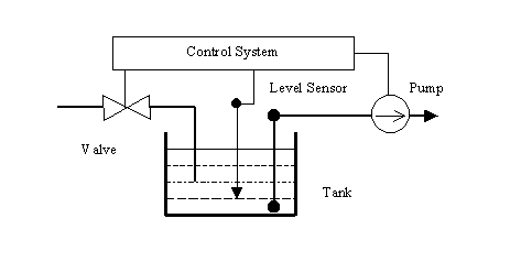
This section is devoted to presentation of a diagnostic example of simple single-tank system.

Diagnostic Problem

For illustration, let us assume that the partial state representation is a logic-like formula of the form  for normal operation, where the meaning of is that the level of the water is higher than some level denoted with low and lower than the one denoted with high.

Now let us consider a formula describing all the states (a situation in our terminology, i.e. a set of states) in which overflow occurs. The formula may be of the form . The failure detection problem consists in checking if the current state belongs to the failure situation. This can be done by formulae matching with respect to their generality; a more general formula describes a bigger set of states. Assume that the level denoted symbolically as very_high is higher than the one of max (in practical system these may be just ordinary numbers). Let the current state formula be , where  denotes the rest of the fats true in the particular state. Thus in our case

In fact, in any state described with the right hand formula above , the failure characteristics specified by the formula  must hold; the crucial element of the check consists in verifying that .

The list of symptoms considered with respect to the example is as follows; they are structured into elementary diagnoses, intermediate symptoms and failure manifestations.

Manifestations, here single failure symptom:

m -- water pouring out of the tank,

Intermediate symptoms:

v1 - valve_open,

v2 - pump_off,

v3 - valve_stuck_in_open_position,

v4 - valve_open_by_control_signal,

v5 - pump_off_by_power_off,

v6 - pump_off_by_control,

v7 - pump_blocked,

v8 - pump_on_by_control,

v9 - valve_open_signal_operating,

v10 - pump_on_signal_from_level_sensor_operating,

v11 - pump_on_signal_from_control_system_operating,

v12 - power_off,

v13 - valve_open_signal_from_level_sensor_on,

Input symptoms - elementary diagnoses:

d1 - valve_stuck_in_open_position_fault,

d2 -valve_open_control_signal_on,

d3 - level_sensor_on_when_level_too_high,

d4 - pump_on_by_control,

d5 - pump_broken_fault,

d6 - power_on.

As one can see, the intermediate symptoms include ones observable (e.g. v2, v5) and non-observable (e.g. v3). Some of the symptoms may be ``artificially'' introduced to assure clear presentation of the graph and protecting distinction between node types (e.g. v10, v11) (avoid type mixing). The initial symptoms cover both elementary diagnoses referring to element faults (e.g. d1, d3), as well as faulty control signals (e.g. d2, d4) and external conditions (e.g. d6).

The causal graph is constructed by analysis of causal dependencies among symptoms and encoding them with node structures. The selection of AND, OR, and NOT nodes helps to express most common phenomena referring to logical functions. NOT nodes are also used to represent symptoms negations. The structure of the causal graph is presented on the figure below.

[here: grapf1.eps

On the picture symptoms (nodes) found to be true are marked with filled circles; the empty circles denote false symptoms or ones of unknown status. After identification of the failure, only the node marked with m is found to be true. When further observations are accessible, also v2 and d6 are marked true.

In order to present the elements of diagnostic reasoning let us consider a particular diagnostic problem, e.g. one given by  and , i.e. the overflow of water when the system is switched on and the pump is observed not to work. The problem is to find diagnoses explaining m and consistent with the observations.

Before we start the analysis, let us propagate the observations through the graph. In fact, only d6=true can be propagated. We obtain v12=false and v5=false; this information can be used for checking consistency with hypothesized diagnoses.

Let us start the analysis from the failure manifestation. In fact, we perform backward, top-down search. As the symptom meaning a failure m is identified, we search for the possible reasons for that; the search is performed backwards, i.e. we look for possible explanations. With respect to our model there is one conjunctive cause possible, i.e. v1=true AND v2=true. The procedure must recursively explain both the symptoms found. Note that v2=true is consistent with the observations (in other case there would be an inconsistency).

Now for explaining v1=true one can suggest two hypotheses, namely v3=true or v4=true. We follow the latter one leaving the first one for further possible exploration (in the algorithm it is saved on the stack). For explanation of v4=true again we have two possibilities; let assume that we select v13 to be true and thus we must have d3=false as the consequent selection; the process of explaining v1 is stopped here since we have arrived at an initial node being an elementary diagnosis. All the other possibilities of explaining v1=true are left for further possible use, while now the problem is to explain v2=true.

For v2=true there are three possibilities. Note that, however, the first one, i.e. v5=true is inconsistent with observations, so it should be left unexplored. Assume we select the second one, i.e. v6=true. Further on, the only explanation of v6/true is v8=false, which is consistent with the observations. And to explain v8=false we must assume that both v10=false and v11=false hold. This implies d3=false (already found on another way), and d4=false. The final diagnosis is then given by , i.e. the level sensor is faulty and no control signal for setting on the pump is provided while the system is on. The further analysis of the diagnosis may lead to detection of one hard fault (element fault, d3=false), finding one control signal set to 0 (if this is a fault it should follow from a further analysis of the control algorithm for the specific conditions), and one operational condition already observed. Of course, this is only a potential diagnosis, and as such it should be verified, e.g. by checking the level sensor and measuring the control signal value. Moreover, several other diagnoses can be found by exploring the other alternative explanations of symptoms, temporarily left pending for further use.

The set of all possible diagnoses consistent with the observations found by the algorithm is: