7.11 Causal logical graphs for diagnostic reasoning
In this section a general model for causal abductive inference is presented.
The model is based on encoding causal dependencies among symptoms with
logical causal graphs, the so-called AND/OR/NOT graphs. A simple uniform
representation for causal graphs with binary-valued logic is presented.
The nodes of the graphs represents symptoms, formally equivalent to propositional
formulae, and the edges of the graph represent causal relationships. Basically,
the admitted causal relationship can reflect the basic logical operations,
conjunction (AND), disjunction (OR) and negation (NOT). The graph structure
represents the causal dependencies among events. It can be used both for
modelling system behaviour and diagnostic inference.
Once a model of causal dependencies is built and the initial assignment
of observed manifestations to graph nodes is carried out, the diagnostic
procedure can be started. Diagnostic inference is based on abductive inference
taking the form a search procedure applied for the graph. This approach
is more general and powerful than the presented ones and can be considered
to constitute an extension of the fault trees application to diagnostic
reasoning.
Symptoms, logical causal links, and graph structure
In technical terms a symptom is usually used to denote a characteristic
of a system occurring at a time. The key issue for explaining faulty behaviour
in technical systems is the knowledge of causal relationship among
symptoms occurring in the system.
The current status of a symptom can be one of the following three
possibilities, i.e. true (known to occur), false (known
not to occur), or unknown. In this work symptoms are considered
rather as useful linguistic category than as precisely defined logical
term; however, from logical point of view one can often regard them as
described with logical formulae. Further, for representation with extended
set of values, symptoms may be considered as variables taking values from
a prespecified set; in our case the set is just  ,
but if necessary, it can be extended to several elements of arbitrary choice.
,
but if necessary, it can be extended to several elements of arbitrary choice.
Several categories of symptoms may be considered. First, there are external
manifestations,
usually denoting failure symptoms and indicating abnormal or faulty behaviour
of the considered system. They constitute the principal observable output
of the system under diagnosis. The set of manifestations to be considered
will be denoted as  .
.
Second, a set of initial cause symptoms is distinguished. An
initial
cause is a symptom without any visible reason or for which one does
not search for any further cause or explanation. Initial causes can be
divided into several subcategories, e.g. component faults, control actions,
external conditions, etc. All of them are considered as elementary diagnoses.
The set of elementary diagnoses is denoted as  .
.
The third category of symptoms are intermediate (other) symptoms;
these are just any symptoms, observable directly or not, which are neither
manifestations (M) nor elementary diagnoses (D). The set
of such symptoms will be denoted by  .
.
The set of all symptoms will be denoted by N, where 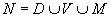 .
Finally, for clarity of the discussion it is assumed that all the three
sets composing N are pairwise disjoint.
.
Finally, for clarity of the discussion it is assumed that all the three
sets composing N are pairwise disjoint.
Taking into account practical diagnostic problems, any element of N
can be regarded as symptom, event, binary variable,
fact
or propositional formula. Thus several ways of notation are possible;
a symptom  being observed
can be denoted as n being true, n=1 or simply n,
while the absence of it can be denoted as n being false,
n=0,
or
being observed
can be denoted as n being true, n=1 or simply n,
while the absence of it can be denoted as n being false,
n=0,
or  .
.
For the sake of graphical representation it is assumed that causal relations
among symptoms are specified with use of graph representation. Any node
of the graph represents a specific symptom .
Whenever there is a causal relation between nodes n and n´,
there is a directed arc pointing from n to n´. The meaning
of the arc is that n causes n´. Using logical notation,
the semantics of a single connection between two nodes is defined n
Æ
n´
i.e. if n becomes true then also n´, necessarily
becomes true. A more detailed definition and some extensions are considered
in \cite{Ligeza:96}, \cite{Fuster:96}.
The nodes of the graph are connected by the so-called functional
components. A functional component connect one or several input nodes
with exactly one output node. A functional component f will be represented
as a triple 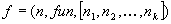 , where n
is
the output node, fun is the performed function and
, where n
is
the output node, fun is the performed function and  are the input nodes. Basically it is assumed that the there are three types
of functional components corresponding to conjunction (AND), disjunction
(OR) and negation (NOT) logical functions. Thus, there are three types
of functional components, i.e.
are the input nodes. Basically it is assumed that the there are three types
of functional components corresponding to conjunction (AND), disjunction
(OR) and negation (NOT) logical functions. Thus, there are three types
of functional components, i.e. 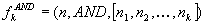 performing logical conjunction on k inputs,
 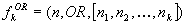 performing logical disjunction on k inputs, and
 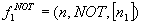 performing logical negation on exactly one input node. For simplicity,
the output nodes corresponding to the functional components are named after
the respective components, i.e. there are AND, OR and NOT nodes, respectively.
performing logical negation on exactly one input node. For simplicity,
the output nodes corresponding to the functional components are named after
the respective components, i.e. there are AND, OR and NOT nodes, respectively.
An AND/OR/NOT causal logical graph is a structure  ,
where N is the set of graph nodes, ,
and F is a set of functional components defining the links between
nodes. Further, it is assumed that there is no arc pointing from the nodes
specified with M (they are tip or output nodes only), i.e. the manifestations
are final nodes, there is no arc pointing to the nodes of D, i.e.
the elementary diagnoses are initial or input nodes only, and there are
no loops in the graph.
,
where N is the set of graph nodes, ,
and F is a set of functional components defining the links between
nodes. Further, it is assumed that there is no arc pointing from the nodes
specified with M (they are tip or output nodes only), i.e. the manifestations
are final nodes, there is no arc pointing to the nodes of D, i.e.
the elementary diagnoses are initial or input nodes only, and there are
no loops in the graph.
Moreover, for the sake of the graph being connected, it may be assumed
that every node has at least one arc pointing to or from this node, etc.
Further considerations and extensions are discussed in [Ligeza
et al, 1996a], [Fuster, 1996].
The interpretation of the above definition is straightforward. There
is a directed arc from node n to node n´ whenever n
causes n´. It is also possible that there are several arcs
pointing from several nodes
to n; in this case the arcs denote a functional element. In this
case the occurrence of any of the symptoms represented by these nodes is
satisfactory for n becoming true, n is referred to be an
OR-node and the arcs (unmarked in any specific way) form the functional
component of type OR. If symptoms
cause n only when occurring together, then all the arcs from
to n are joined by a special ``horizontal'' arc and form a functional
component of type AND; node n then is referred to as an AND-node.
Further, there is an arc labelled NOT from  to n whenever absence of the symptom defined by
(its negation) causes n to occur.
to n whenever absence of the symptom defined by
(its negation) causes n to occur.
An example AND/OR/NOT causal graph is presented in the figure below.
The defined above AND/OR/NOT causal graph is similar in structure to
classical AND/OR graphs used in problem-solving [Nilsson,
1980]. The main differences consist in the direction and interpretation
of arcs (here different extensions of the basic causal interpretation are
possible; see for example the MAY links in [Console
et al, 1989], [Console
and Torasso, 1992]; see also [Fuster,
1996] and nodes -- an initial node here means only possibility
for solution). The application of the graph is also different. A visible
extension consists in admitting the NOT links. Further, a ``solution graph''
in classical problem-solving constitutes only a ``possible justification''
(to be further validated) for the observed failure. The AND/OR/NOT causal
graphs constitute also a refinement of fault trees [Barlow
and Lambert, 1975] and causal graphs used in model-based diagnosis
oriented towards direct search of diagnoses.
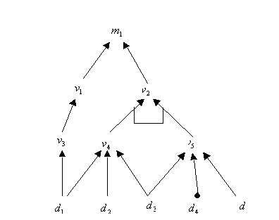
The only AND node is  ,
the link between
,
the link between  and
and  is of type NOT.
The AND/OR/NOT causal graphs seems to constitute a uniform, intuitive
and powerful formalism. In fact they can subsume most of the formalisms
presented so far. As we shall see, the inference procedure is also uniform
and relatively simple.
A diagnostic problem statement and its solution
A diagnostic problem exists if at least one fault is observed. The faults
to be diagnosed are assumed to be specified with some manifestations (either
positive or negative ones). Consider an AND/OR/NOT causal graph G.
Formulation of diagnostic problem takes also into account some possible
observations providing further information to the diagnostic system.
A diagnostic problem is a five-tuple 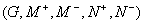 where
where  and
and  are the fault manifestations to be diagnosed, respectively true
and false, and where
are the fault manifestations to be diagnosed, respectively true
and false, and where  and
and  , are the auxiliary
observations specifying which further symptoms are true and false;
there is
, are the auxiliary
observations specifying which further symptoms are true and false;
there is  and
and  ,
while
,
while  and
and  .
.
The sets of manifestations true and false provide the fault definition
and must be explained by all the diagnoses found, while the auxiliary observations
provide information which can be used for guiding, ordering and refining
the search. Further, any diagnosis must be consistent with the observations.
In order to solve diagnostic problem one is to search for a set of possible
initial cause symptoms explaining (justifying) the failures specified with
current manifestation values. Basically, the search for possible diagnoses
(not necessarily the minimal ones) can be any systematic graph search procedure
[Nilsson,
1980] taking into account the specific character of the defined graph
(interpretation of nodes as symptoms; some of them can be known a priori
to be true/false) and its elements (i.e. the AND, OR and NOT connections).
Thus, informally speaking, the problem of finding possible (potential)
diagnoses is equivalent to finding a set (minimal set) of initial symptoms
defining faulty components, control actions and external signals, such
that the combination of initial causes implies the observed abnormality.
In fact, a diagnosis may be any consistent combination of values
of symptoms from D, justifying the observed abnormal behaviour with
respect to the graph structure and consistent with observations.
The search for potential diagnoses is performed in backward manner.
For a given set of manifestations one has to hypothesise and explore possible
status of former nodes implying the observed status of manifestations.
Let us recall that any node can take one of the following states: be known
(or assumed) to be true, be known (or assumed) to be false
or be
of unknown status. The current assignment of truth-values to
symptoms in the graph (possibly not to all of them) determines the current
state of the search.
Formally, in order to define state of the search, we introduce a mapping
of the form: 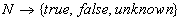 assigning
to any symptom its current status. In practice, the initial state of the
search is defined by specification of the manifestations true and false
( and )
and the observations of true and false symptoms (
and ). During the search
some new nodes are supposed to become true or false; thus, at any stage
of the search the set of nodes true is of the form
assigning
to any symptom its current status. In practice, the initial state of the
search is defined by specification of the manifestations true and false
( and )
and the observations of true and false symptoms (
and ). During the search
some new nodes are supposed to become true or false; thus, at any stage
of the search the set of nodes true is of the form  (where
 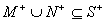 ) and the set of
nodes false is of
) and the set of
nodes false is of  (where
 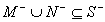 ).
).
Symptoms of the value unknown are not represented explicitly
in state set. Further, it is assumed that any state defined with
and is consistent, i.e.  - the intersection of true and false symptoms is empty. Moreover, we shall
also assume that any state set is maximal with respect to the possibility
of information propagation. Whenever some new node is evaluated or assumed
to be true/false, this information influences the state of the search.
The rules of propagation are defined below:
- the intersection of true and false symptoms is empty. Moreover, we shall
also assume that any state set is maximal with respect to the possibility
of information propagation. Whenever some new node is evaluated or assumed
to be true/false, this information influences the state of the search.
The rules of propagation are defined below:
Forward propagation: (causality, simple logical interpretation
assumed)
OR node true: if at least one of the predecessors of an OR node
is true, then the value of the OR node is set to true,
AND node false: if at least one of the predecessor of an AND node
is false, then the value of the AND node is set to false.
NOT node true: if a predecessor of a NOT node is false, then the
value of the NOT node is set to true,
NOT node false: if a predecessor of a NOT node is true, hen
the value of the NOT node is set to false.
Forward propagation: (causality, simple logical interpretation
assumed; further, the predecessors of a node are assumed to be all the
direct causes for it)
OR node false: if all the predecessors of an OR node are false,
then the value of this OR node is set to false,
AND node true: if all the predecessors of an AND node are true,
then the value of this AND node is set to true.
Backward propagation: (causality, simple logical interpretation
assumed)
OR node false: if an OR node is false, then the values of
all its predecessors are set to false,
AND node true: if an AND node is true, then the values of
all its predecessors are set to true,
NOT node true: if a NOT node is true, then the value of its
predecessor is set to false,
NOT node false: if a NOT node is false, then the value of
its predecessor is set to true.
Backward propagation: (causality, simple logical interpretation
assumed; further, the predecessors of a node are assumed ton be all the
direct causes for it)
OR node false: if an OR node is false, then all the values
of its predecessors are set to false,
AND node true: if an AND node is true, then the values of
all its predecessors of are set to true.
The above rules define the principles of state propagation. Whenever
a rule is applicable, a new symptom value is generated; it is next placed
in the set representing current state. In case some symptom turns out to
take two inconsistent values, the initial state for propagation is considered
to be inconsistent and it is not taken into account any more. In practice,
this has the effect of failure and backtracking in Prolog.
Now, let  be any set
of input symptoms together with their values, where
be any set
of input symptoms together with their values, where  specifies which symptoms are true, and
  gives false symptoms. Further, let
  denote a state of the graph providing the set of symptoms true and false,
respectively. The state specified by
is said to follow from (or be implied by)
iff it can be generated from
with respect to the above propagation rules; this will be denoted as
Ã.
denote a state of the graph providing the set of symptoms true and false,
respectively. The state specified by
is said to follow from (or be implied by)
iff it can be generated from
with respect to the above propagation rules; this will be denoted as
Ã.
An initial change of node status is the result of failure detection;
the appropriate nodes belonging to M change their status from unknown
to true or false. Further changes of the current state of
the graph can be performed as a result of the following operations:
assumption, i.e. hypothesis formation concerning certain node performed
by graph-search procedure; this change is always from unknown to
true/false,
performing a test, i.e. probing (or just observation); a test assigns values
true/false
to one or more nodes,
finally, after any such change the propagation rules are applied so that
all possible changes are performed,
last but not least, if after that the new state is inconsistent, some assumption
about symptom status must be withdrawn (backtracking) so that consistency
is regained.
With respect to the definition of an AND/OR/NOT causal graph and
the diagnostic problem, a solution to the problem is any consistent combination
of the values of initial causes, such that it implies the observed malfunctions.
The maximal state implied by a diagnosis must be internally consistent,
and it must be consistent with observations.
Let , denote a diagnostic
problem. A possible diagnosis constituting a solution to the diagnostic
problem is any (minimal) pair of sets
of all the initial nodes true and false such that the following conditions
are satisfied:
à  .,
i.e. the diagnosis implies the observed manifestations,
if describes the maximal
state implied by and the
observations, then
.,
i.e. the diagnosis implies the observed manifestations,
if describes the maximal
state implied by and the
observations, then
i.e. the maximal state following from a diagnosis and observations
must be consistent,
According to the above definition a diagnosis is assumed to be minimal,
i.e. no pair of subsets of it is a diagnosis; one can also consider non-minimal
diagnoses, or diagnoses minimal with respect to induced subgraph of [Fuster,
1996], [Ligeza et al, 1996a].
An illustration of example solutions for the problem specified with
a graph presented above as an example. Assume the diagnostic problem is
given by  , i.e. the only
manifestation is true. In the figure below there are possible solution
graphs; the presented three graphs constitute possible solutions
for the assumed failure. The bottom nodes constitute possible potential
diagnoses.
, i.e. the only
manifestation is true. In the figure below there are possible solution
graphs; the presented three graphs constitute possible solutions
for the assumed failure. The bottom nodes constitute possible potential
diagnoses.
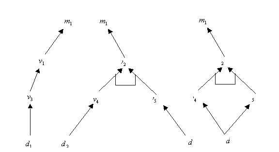
For intuition, there are four minimal diagnoses, i.e.  ,
,  ,
,  and
and  ; the first three are
presented in the picture.
; the first three are
presented in the picture.
The search for solution is performed by a backward search procedure
selecting and hypothesising the state of predecessor nodes so that the
state of the problem defining nodes is explained. The following points
specify the rules of backward search in case of AND, OR and NOT connections
used:
OR node true: explained by selecting*
one
of its predecessors and setting it to true,
AND node true: explained only by setting all of its predecessors
to true,
OR node false: explained only by setting all of its predecessors
to false,
AND node false: explained by selecting*
and
setting one of its predecessors to false,
NOT node true: explained by its predecessor being false,
NOT node false: explained by its predecessor being true,
initial nodes: initial nodes are set to true or false when
necessary; arriving at an initial node completes the search on the selected
path.
The operations are performed only if they do not lead to inconsistency.
The node selection procedure may be systematic, indeterministic, or heuristic
one. Since the algorithm always select a single node in the case of OR
node true and AND node false, the generated solutions are, in general,
minimal.
Note that with respect to the definition, a solution to diagnostic problem,
i.e. a diagnosis, constitutes in fact a possible explanation of the observed
failures; in order to verify it in practice one should test all its elements.
Validation of generated diagnoses is the next step of diagnostic procedure.
Validation of diagnoses
With respect to the model of diagnostic knowledge representation in the
form of an AND/OR/NOT causal graph, any of the generated diagnoses constitutes
a sufficient explanation of the observed faulty behaviour. However, usually
only one of the diagnoses is the valid one, i.e. the one defining real
troubles in the diagnosed system. In fact, validation of the obtained
candidate diagnoses in order to identify the correct one should be performed.
Validation can potentially be done by simulation of the influence of the
hypothesised elementary faults on the observable behaviour of the system;
however, this would require a more complete model of the system, covering
abnormal behaviour, so that all but one of the potential diagnoses can
be eliminated. This, however, is hardly possible in real cases. Thus the
principle method consists mostly in testing the potential elementary causes
in direct or indirect manner.
For obvious reasons minimal diagnoses are preferred to the other ones.
This point of view reflects the most natural tendency to find as simple
explanations as possible. principle of parsimony. The problem of
efficient validation of the final set of possible diagnoses is considered
below in brief.
Let us assume that after a systematic search of the causal graph a set
of a set of k possible diagnoses is obtained. Any of these diagnoses
is of the form  , where
  .
Note that any diagnosis
is assumed to be minimal and consistent. In case consideration of minimal
diagnose is not sufficient, all superset diagnoses should be further considered.
.
Note that any diagnosis
is assumed to be minimal and consistent. In case consideration of minimal
diagnose is not sufficient, all superset diagnoses should be further considered.
A strategy for validation of diagnoses can be built on a number of assumptions
and additional knowledge (e.g. the use of probabilities and minimisation
of entropy). Here a strategy based on heuristic approach is proposed. The
main idea is to separate the set of currently considered diagnoses into
two almost equal, disjoint sets as a result of a test of one symptom, being
a common element of the diagnoses.
In the following part, a test is assumed to be an algorithmic procedure
providing the truth value of a single symptom being an element of some
diagnoses. A test can confirm a diagnosis if the tested symptom included
in a diagnosis is found to have the status identical to its status in this
diagnosis; in the other case, the test rejects current diagnosis.
A diagnosis is contradictory
to diagnosis  if and only
if
if and only
if  or
or  ;
an element d belonging to such intersection will be referred to
as a conflicting element with respect to diagnoses the above diagnoses.
Since the result of testing is unknown a priori, it is heuristically justified
to test first conflicting elements - no matter what the result of the test
is, at least one of the diagnoses is rejected. The "most useful" test is
one rejecting the maximal number of diagnoses at a time. The number of
rejected diagnoses is, however, unknown a priori. Thus, the following heuristic
approach based on "almost equal partitions" is put forward.
;
an element d belonging to such intersection will be referred to
as a conflicting element with respect to diagnoses the above diagnoses.
Since the result of testing is unknown a priori, it is heuristically justified
to test first conflicting elements - no matter what the result of the test
is, at least one of the diagnoses is rejected. The "most useful" test is
one rejecting the maximal number of diagnoses at a time. The number of
rejected diagnoses is, however, unknown a priori. Thus, the following heuristic
approach based on "almost equal partitions" is put forward.
Let  denote the number
of occurrences of d in the positive parts of diagnoses
denote the number
of occurrences of d in the positive parts of diagnoses  ,
where . Respectively, let
,
where . Respectively, let  denote the number of occurrences of in the negative parts of the diagnoses
  ,
where . Thus, the least
number of diagnoses rejected after a test of element d, to be denoted with
r(d),
can be determined as
,
where . Thus, the least
number of diagnoses rejected after a test of element d, to be denoted with
r(d),
can be determined as
 and the proposed selection of element(s) d to be tested should maximise
r(d).
and the proposed selection of element(s) d to be tested should maximise
r(d).
Let  denote the symptom
selected to be tested first; there should be:
denote the symptom
selected to be tested first; there should be:
 In case the selection of
is not unique, further heuristic of cost criteria can be taken into account.
Again, having sufficient knowledge about underlying probabilities, the
above test can be generalised so as to select a test rejecting the maximal
expected or average number of diagnoses.
In case the selection of
is not unique, further heuristic of cost criteria can be taken into account.
Again, having sufficient knowledge about underlying probabilities, the
above test can be generalised so as to select a test rejecting the maximal
expected or average number of diagnoses.
