1

4.6 Decision lists, decision tables, decision trees In this section three simple tools for encoding decision procedures are outlined in brief. These tools are decision lists, decision tables, and decision trees. Any of them is aimed at providing operational support for efficient decision making. Any of them introduces a specific structure into the decision process and allows for algoritmization of decision procedures. Although the tools are relatively simple, they allow for multilevel hierarchical decision making and thus can be used for encoding quite complex decision support procedures. Decision lists Decision lists are one of the conceptually simplest tools for encoding process of decision support. A decision list is composed of a sequence of pairs (binary condition, action). Its use consists in sequential checking of the list items, and every time when the condition is satisfied, the appropriate action is executed; then next pair is examined.

Note that from logical point of view, the conditional part is just a proposition logic atomic formula, and thus it is evalueted to true (T) or false (F). Its definition is usually formulated as a question concerning status, position, current state, etc. of some switch, device, item or object. Depending on the answer, an asigned action is executed or not.
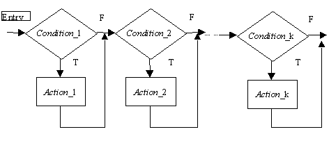
There can be two basic oragnizations of decision lists. The first one is simple linear; in such an organization the conditions are examined in turn, every time when the condition is evaluated to true the appropriate action is executed; then the next condition is evaluated, etc. Thus, in linear organization every condition is evaluated once and all the list is scanned along disregarding if any actions (and which) were executed. A graphical scheme of such a list is presented below.

A linear decision list
After entering the list, the first condition is evaluated. If it is true (T), the first action is executed. Disregarding the results and the condition value, the following condition is evaluated next, etc. After coming to the end of the list, either the scanning proces can be repeated (in a closed loop) or the operation can be terminated. Initiation of the entry to specific decision list can be the result of execution of some higher order prcedure or satisfaction of some entry conditions. The actions may represent real operation on the supervised system, decisions, or just certain conclusions to be inferred.
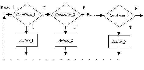
Another possibility of organization of a decision list consists in hierarchical structure. The principle is that the most constrainng condition (the strongest one, the most important one) is evaluated first, and if found to be true, the appropriate action is executed; the list is abandoned and, possibly, interpreted once again from the beginning. If the first condition is false, the following conditions are evaluated sequentially until encountering the first one true. Then the appropriate action is executed and the list is abandonned. This king of organization is schematically presented in the figure below.

A hierarchical decision list.

The main applications of linear decision lists take place in situations where more or less equally important conditional activities are to be performed sequentially, and perhaps in a closed cycle; this includes routine checking of some external conditions, specification of simple reactive systems, etc. On the other hand, hierarchical decision lists are applied mainly for encoding conditional actions ordered according to some priorities, i.e. an action of higher priority should be always executed before and action having lower priority, provided that their conditions are satisfied.

Decision trees A useful, engineering way of knowledge representation for decision making may consist in further structuring the knowledge with use of different tree-like representations. Thus a decision tree can be considered to be an extension of decision lists concept.

Tree-like representation are readable, easy to use, and generally accepted structures displaying in an intuitive form some decision or classification procedure. The root of the tree is the entry node, and under any node there are some branching links. The selection of a link is carried out with respect to a conditional statement assigned to the node. Evaluation of this condition (either to true or false in case of binary trees, or to one of prespecified values in case of more complex trees) determines the selection of the link. The tree is traversed top-down, and at the leafs final decision or classified object are encountered.

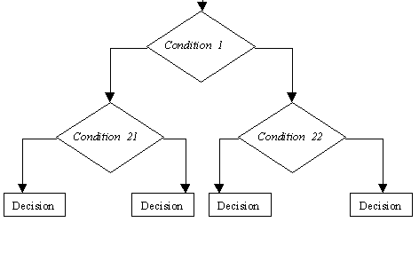
The basic form of decision tree is a binary decision tree. Any node in such a tree (apart from leaf nodes) is assigned a binary condition equivalent to a propositional formula. Below any such node there are normally two branches, one corresponding to the sequence of traversing the three is the assigned condition is true (T) and the other one corresponding to the case when the condition is false (F). A graphical scheme of such a tree is outlined below.

A simple binary decision tree.

A decision tree may have nodes corresponding not only to binary branching. For example, a node may be assigned a question concerning the value of certain attribute, and there may be as many links going out of this node as many possible values for the specified attribute exists. For practical reasons the number of possible branches is usually limited to just several. Decision trees can be also organized in a hierarchical way, i.e. the leaf node of an iupper level decision tree can be the root node for a lower level decison tree.
In particular, in certain cases a decision tree can take the form of of a decision graph, i.e. certain branches are linked together in order to avoid specifying the same questions in the same or similar situations for many times. It is important, however, that a decision tree is always traversed top-down, ie. even if it takes the form of a graph, no cycles can be introduced.

Decision tables Another similar idea is a decision-table. A decision table is a table displaying sequences of conditions which must hold for executing specific actions. The sequences of conditions are displayed in a readable form, either vertically, as parts of columns of the decision table, or horizontally, as parts of row of the table.

A classical form of decision table is the vertical one. where condition_i specifies the conditions to be examined, and action_i defines the action to be executed. The values v_ij can take + if the condition must hold for certain action to be executed, -if the condition cannot hold (if it holds, then the action cannot be executed), and * (or empty place) which means that the action is condition-independent. The values w_ij take + if the action is to be executed, provided that the vertical condition-defining sequence above is satisfied, or - (or empty space) if the action need not be performed. A generic for of such a decision table is presented below.

condition_1	v_11	v_12	v_1n
condition_2	v_21	v_22	v_2n

condition_k	v_k1	v_k2	v_kn
action_1	w_11	w_12	w_1n
action_2	w_21	w_22	w_2n

action_m	w_m1	w_m2	w_mn

The evaluation of the table proceeds as follows: any column of values specifying action prerequisites is traversed top-down, and the defined sequence of true and false conditions is verified. If the pattern is matched, the actions specified below are executed, and subsequent column of conditions is analyzed. In stable environment, the conditions can be evaluated once for processing of all the table, and then only conditional sequences are matched against the current pattern of true and false conditions.

The main advantage of a table as above consists in simple, intuitive interpretation. Further, the evaluation procedure can be speeded up due to singular evaluation of conditions during each cycle. Furthermore, tables can be organized in a hierarchical manner, i.e. certain action may consist in going to analysis of a lower order, more specific table (an action similar to the ''go to'' instruction in some programming languages). One of the main disadvantages consists in possibility of defining the preconditions of actions with use of binary values only, and in some cases the use of values of attributes is more convenient. A slightly extended table, the so-called Object-Attribute-Value Table (OAV Table, OAT) is presented below.

attrib_1	attrib_2	attrib_k	action_1	action_2	action_m
v_11	v_12	v_1k	w_11	w_12	w_1m
v_21	v_22	v_2k	w_21	w_22	w_2m

v_n1	v_n2	v_nk	w_n1	w_n2	w_nk

The OAV table is very similar to relational database table, and in fact it is a RDB with specific interpretation of certain columns. The basic scheme is presented below.
In the above table, the rows specify under what attribute values certain action must be executed. Since both v_ij and w_ij may take many different values (not just true/false, or unimportant, as in the former case), the approach is more general than the former, classical table. In case of actions, the specific values may indicate if the action is to be applied or not, but they can also specify some parameter of the action associated with specific column. The
interpretation (and execution) of this table is straightforward: the rows are examined in turn, and the current values of subsequent attributes are determined; if they match the pattern specified in the examined row (i.e. the specification given in the examined row is more general than the provided current specification), the actions specified in the right-hand part of the table are executed, and next rows is examined. Of course, hierarchical organization of tables is also possible.