4.11 Graphs and causal graphs
Various sorts of graphs are popular means for knowledge representation
in Artificial Intelligence. A basic notion of a graph is as follows. Consider
a set of nodes ,N, which represent some entities; these can be events,
propositional statements, symptoms, variables or even complex frame-like
structures, theories, etc. Amongst the nodes various types of relationship
can take place; in the basic formulation one can consider just one type,
such as causality, logical entailment, physical dependency, etc. The relations
among nodes are represented with arcs (links), and can be directed (one
way) or undirected (symmetrical). The relation, to be denoted R,
is a subset of the Cartesian product. The graph is defined thus as a pair  ,
,  .
.
Depending on the particular application, various modifications of the
basic definition are possible. Generally speaking, there can be several
different types of nodes admitted, and several different types of links
among them. Some links can take more complex, functional form and they
can link several input and several output nodes. Further, various interpretations
of nodes and links are possible.
This section is devoted to presentation of selected basic graph based
models with special attention paid to models incorporating various
forms of causal graphs. There are quite a number of approaches based
on the intuitive notion of causality and graphical representation of causal
dependencies among symptoms (events, variables, nodes). Some most typical
representations are sketched out below. In Chapter 7 a more general model
covering most of the presented one and based on logical causal graphs will
be presented.
Fault trees
One of the earliest use of causal graphs in systems engineering consisted
in analysis of safety and reliability with use of the so-called fault trees
[Barlow
and Lambert, 1975]. Fault tree analysis (FTA) has been for quite a
long period now recognised and industrially accepted technique for dealing
with complexity of systems while analysing its safety and reliability.
The origin of FTA dates back to early sixties and first applications in
the aerospace industry. This widely applicable technique can be used in
diversity of fields including complex, heterogeneous systems as e.g. nuclear
power plant. It is mainly applied to safety analysis, but can also be used
in diagnosis for predicting the most likely causes in the event of a system
breakdown, and as such it may be of interest in supervision for prediction
and decision support. It forms also some bases for diagnostic models.
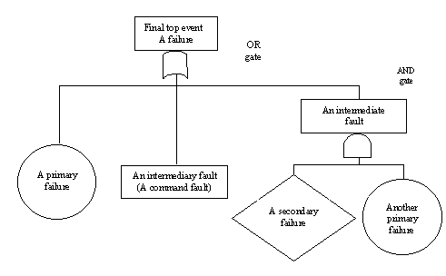
A fault tree consists of nodes representing events in the system
and logic gates, usually AND and OR, for representation of relationship
between events. Typically, four types of events are distinguished:
-
fault events, represented with rectangles
referring to both faults and normal events and being outputs of the logic
gates (basically OR and AND ones).
-
basic events, represented with circles O
referring to inherent failure of some system element (primary or generic
failures),
-
undeveloped events, represented with diamonds à
referring to other than primary failures, purposely not developed further,
-
switch events, represented with Ù
put over ë
û
and summarising some events expected to occur or never occur because of
the design and normal conditions.
The events are connected with arrow links by use of the selected
logic nodes; an OR node represented the disjunction of conditions causing
the output to occur, while an AND node represents the conjunction of conditions
causing the output to occur. A simple example of a fault tree is presented
on the figure below.

Other example fault trees and their construction and use are
described in [Barlow and
Lambert, 1975]. More complex fault-symptom trees, covering the possibility
of using fuzzy fault evaluation are presented in [Isermann,
1994].
The fault trees model [Barlow
and Lambert, 1975] can be used in a variety of ways for analysing system
safety. The possible approaches include fault simulation, analysis of fault
propagation, probabilistic safety assignment, and diagnostic inference.
Below we present a simple algorithm useful for identification of possible
causes for observed malfunction of the system. the procedure is called
minimum
cut set algorithm.
A cut set is a set of basic events such that simultaneous occurrence
of these events causes the top event of the tree to occur. A cut set is
minimal if no proper subset of it causes the occurrence of the top event.
For a single top event there may be several different minimal cut sets.
A list of all minimal cut sets - if determined - can be helpful in analysing
safety, identifying possible or potential causes of a failure and - possibly
- redesigning the system to achieve proper level of safety.
The basic principle of the algorithm consists in backward analysis of
potential causes for a selected top event. Note that, in case of OR gate
there are several alternative causes, while in case of an AND gate there
is one cause but composed of several simultaneous events. Thus, an OR node
always increases the number of possible cut sets constructed during the
analysis, why an AND node increases the size (the number of elements) of
the cut sets. The algorithm proceeds top-down in a recursive mode. When
primary event are the only ones remaining, the algorithm stops; the most
recent sets are the minimal cut sets for the tree.
The principal scheme of the algorithm can be expressed with
the following rules:
-
start with the top node, and proceed top-down in a recursive manner; the
temporary working solution is a list of alternative cut sets (conjunctive
causes), initially empty,
-
for any node which is an OR node build a list of alternative causes corresponding
to the input nodes,
-
for any node which is an AND node build a single list of causes containing
all the input nodes,
-
at any stage replace at least one non-terminal node with appropriate construction
according to the above rules,
-
if an OR node appears under an AND node, reduce the resulting working solution
to the form of a list of cut sets by creating a separate cut set for any
input node of these OR node,
-
if all the nodes correspond to primary cause stop; remove non-minimal cut
sets.
Finally, the generated cut sets are the ones which are only minimal.
The algorithm systematically develops all the potential cut sets. Note
that from logical point of view the idea of this algorithm can be explained
as development of a minimal DNF formula implying the top node.
Simple directed graphs
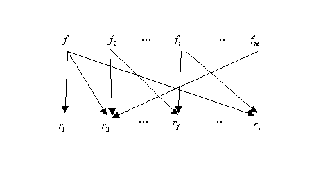
Simple directed graphs represent mutual relationship between faults and
residuals. A basic construction constitute a two-level graph, where the
upper level consists of possible faults  and
the lower level consists of possible residuals (observations)
  The faults point to residuals which are (normally) observed if the fault
is present. This kind of simple graphs is discussed in [Frank,
1994] and [Frank, 1995]. A schematic
representation is given on the picture below.

Note that a graph as above can be equivalently represented
by a set of rules
of the form:
 if fault
=
 then
residual =
where the number of rules is equal to the number of links in
the graph. Further, the representation can be crisp (classical case) and
fuzzified, as in [Frank, 1994] and
[Frank,
1995]. Below two particular formalism using this paradigms are outlined.
However, for practical application purposes, the interpretation of the
graph with inference rules is usually upward the direction of causality.
This means that the diagnostic rules take the form:
 if residual
=
 then
fault
=
 is possible
i.e. the occurrence of a residual is an indication of a specific
fault. Further, combinations of common presence of residuals can be interpreted,
and fuzzy inference rules can be applied.
Diagnostic relations and Kö
nig's bipartite graph
Following the above considerations, below a basic classical formulation
of diagnostic problem, based on the use of diagnostic relation.
Despite some changes in symbols used in the description the formalism is
based on [Koscielny, 1994] and
[Koscielny,
1995].
A finite, discrete set of possible faults is considered. The set is
denoted as  . The elements
of D are also referred to as elementary faults or elementary
diagnoses. They denote elementary final findings in the diagnostic
process, such that the assumption of them entails the observed misbehaviour.
From functional point of view they cover component faults, control/operator
decisions and external events. They can be also considered as input
symptoms if causal interpretation is considered.
Further, a finite set of manifestations is assumed to be specified.
The set is denoted as  .
Manifestations are the outermost findings used to detect failure occurrence
and start the diagnostic procedure; they are also referred to as diagnostic
tests
or observable failures. They can be also considered as output symptoms
if causal interpretation is taken into account.
Elements of D and M can be interpreted as symptoms
or events; from logical point of view also as propositional formulae.
In the basic model it is assumed that both of them can take only two values,
i.e. 0 if the symptom does not occur and 1 if it is observed to be true.
A diagnostic relation is the core model used for fault isolation;
it is of the form  . The
meaning of
 is that elementary
fault
  is the cause of
manifestation
  , i.e. if
  holds them
  is observed.
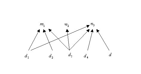
The diagnostic relation  can be represented in the form of diagnostic matrix (a binary one)
or in the form of Kö nig's bipartite
graph [Koscielny, 1994]} and [Koscielny,
1995]; the graph is denoted also as
  .
.
An example graph is presented in the figure below.

The diagnostic procedure consists in fault isolation. For known
values of manifestations one is to find all the (minimal) subsets of the
set of elementary diagnoses, such that assuming them to occur constitutes
a satisfactory explanation of the observed configuration of manifestations.
Thus a diagnosis is any (minimal set  ,
such that
  where
where  is the observed manifestation pattern to be explained with a diagnosis.
For example, if the observed manifestation pattern is defined as
  ,
then the minimal diagnoses are
  ,
,  and
and  . Under assumption
of a single fault the only diagnosis is
  .
.
The diagnostic algorithm constitutes a simple but specified abductive
inference. It can be performed in many ways, including systematic evaluation
of all the subsets of D; in such a case it would be reasonable to
start with single-element subsets of D, and stop the analysis for
any subset which would cause more than the observed manifestations; of
cause, for a generated solution causing exactly the observed manifestations
no proper superset is to be analysed as well.
A more efficient algorithm may consists in abductive analysis of the
set of observed manifestations. The following rules summarise the principal
idea:
Set covering model
Another similar model is the one based on set covering, initially proposed
in \cite{Reggia:83}. A diagnostic problem is understood there as one specified
with a set of abnormal findings, i.e. manifestations and it is required
to explain their presence with another set of disorders, i.e. elementary
diagnoses. Let M denote the set of all possible manifestations (the
potential ones) and D the set of potential elementary disorders.
It is normally assumed that  .
Further, the causal relationship among disorders and manifestations is
captured with some relation
  ,
where
  means that
  can cause
  . One should
note that in this case the relation is a non-deterministic one, i.e. the
presence of
  does not necessarily
implies that
  is observed.
In other words, the causation is a weak one or of the type may.
Given the two sets and the causal relation one can define the
following sets:

and

for any  and
and  .
The first set,
  denotes
all possible manifestations caused by specific disorder, while the second
one, i.e.
  denotes all
alternative disorders that can cause specific manifestation.
Finally, let there be given a set of observed manifestations,  ,
such that
  . The diagnostic
problems consists in explaining the manifestations of
  .
A diagnostic problem is thus specified by a four-tuple
  .
.
Now one can look for all possible explanations. Obviously, it is convenient
to consider only minimal ones, i.e. such that no subset of them is an explanation
of the full set of observed manifestations. Thus, given a diagnostic problem,
an explanation is a set  ,
such that
  (i.e. D´
covers or fully explains
  )
and such that there does not exist any other explanation D´´
satisfying the above condition and such that
  ,
i.e. D´ is minimal with respect to set inclusion. The presented
definition is slightly more general than the one of [Reggia
et al, 1983]; in the original paper minimal solution with respect to
the number of elements (cardinality) are preferred.
Note that, in this kind of model is quite similar to the former one
based on diagnostic relations. The principal difference consists in admitting
weak causality. As the result, one can expect a greater number of potential
diagnoses, since the potential diagnoses are not limited to the ones ''exactly
fitting'' the observed manifestations.
Note that the solution - in general case - is not necessarily unique;
several sets, incomparable with respect to inclusion relation can form
minimal explanations. Let us consider the diagnoses generation problem
as a specific case of abductive inference. For any manifestation  one has to look for a disjunctive list of possible causes. By examining
the observed manifestations in turn, several such sets are generated. Any
time a new set is generated it is to be combined with the temporary solution
exactly as in the former model. Non-minimal solutions are simply removed.
Any final set of initial causes fully explains the observed manifestations,
and is minimal. It can, however, contain primary causes being potential
causes of other manifestations, which are not observed in the current state
of the system.
Signed directed graphs - SDG
This kind of causal graphs were established to model continuous processes.
The basic idea of the technique consists in tracing the observed malfunctions
back to their origin. To enable this process one needs to represent possible
ways and types of information propagation. The proposed model takes the
form of signed directed graph (SDG) and was proposed by Kramer and
Palowitch; a presentation based on the original paper can be also found
in [Tzafestas, 1989].
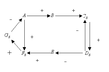
A signed directed graph consists of nodes which represent state
variables, alarm conditions, fault sources or sensor-measured values, and
branches (edges) representing the influence between nodes. The influence
can be positive (marked with '+') or negative (marked with '-' over the
edges). A node can influence several other nodes. Any node can be influenced
by none, one or several nodes. Auxiliary information can also be specified;
it may include time delays, intensity of the influence, probabilities,
etc.
The representation is somewhat oversimplified but very intuitive, and
for supervision and diagnostic inference can be quite satisfactory in many
cases. However, in order to assure correct work, several limiting assumptions
must be accepted:
correct diagnosis can be obtained only if each variable undergoes at maximum
one transition between qualitative states during fault propagation; in
fact, a steady-like state is analysed, where the variables change from
normal to abnormal value along the propagation path,
single fault influencing single root node is assumed to be the source of
all perturbations observed,
occurrence of the fault does not change other causal pathways in the graph.
The causal graph can be used both for fault modelling (i.e. simulation
of fault propagation) and diagnosis (i.e. searching for initial causes
of the observed malfunctions). In fact, the two activities are close to
dual (or inverse) tasks. Assuming fault of a single node is necessary to
provide the possibility of generation of directed trees showing the propagation
of the fault. From a single node several trees can usually be generated.
Any such tree constitutes an interpretation of fault propagation. Normally,
only one of the trees (or a part of it) shows the actual paths of fault
propagation, the other refers to possible interpretations presenting potential
behaviour possibilities. Fault propagation involves construction of all
such tree representing possible fault propagation. Diagnostic task consists
in identifying all root nodes being provided with sensor-obtained qualitative
values of system variables. The typical choice of these values consists
of high (+1), normal (0) low (-1).
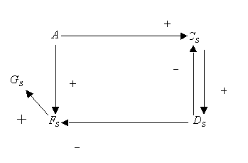
Consider a simple graph presented on the figure below.

Assume that the fault enters the network at the A node
changing the variable value from normal (0) to high (+1).
Assuming that nodes B and E are unmeasured ones, one can
further simplify the initial graph to the form presented below, by node
lumping procedure; this procedure 'eliminates' all unmeasured variables,
as ones of no interest (except as potential root nodes, which is not the
case here). In fact, such nodes provide no new verifiable information.
Further, the link from  to A was removed, since by assumption the positive perturbations
is strong enough to override the negative feedback.
The resulting simplified graph is presented below.

Note that the graph still contains one loop with negative feedback.
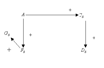
Now consider the possible ways of fault propagation. First, the fault can
propagate from A to  and further to
  . Simultaneously,
it can propagate from A to
  and, through the loop, to
  .
Due to the assumption of single state transition, C cannot return
to normal value by the negative feedback in the loop. Similarly,
in this interpretation
  cannot be changed to low or normal by negative influence
of
  .
.
This interpretation is show below.

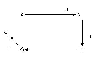
Another possibility consists in propagation of the fault from
A
to  through
  ,
,  ,
and
,
and  . Note that on the
path one negative influence is present.
The interpretation is show on the picture below.

In the development of interpretations one traces down paths
from the root node to leaf ones, keeping consistency with the assumptions
(no variable can change twice or more), and taking into account the direction
and sign of the edges. Feedback loops are typically removed by assuming
that they cannot compensate fully for the perturbation.. However, in certain
cases this may be not true; then, interpretations taking into account the
negative feedback effect possibly cancelling the disturbance on the controlled
variable.
The interpretation trees define possible patterns of steady-state
like fault occurrences. The fault, observed as perturbation of the variable
value can propagate only down the tree, from the root node, according to
the signs of edges. It can stop at some variables before reaching the leafs,
however, due to the assumption there cannot be a gap in the path of fault
propagation: if certain variable on a selected path is disturbed, then
all the ancestor variables must be influenced as well. For the two interpretations
presented above, the fault propagation patterns are as in the two following
tables,
 |
 |
 |
 |
| 0 |
0 |
0 |
0 |
| 1 |
0 |
0 |
0 |
| 1 |
1 |
0 |
0 |
| 0 |
0 |
1 |
0 |
| 0 |
0 |
1 |
1 |
| 1 |
0 |
1 |
0 |
| 1 |
1 |
1 |
0 |
| 1 |
0 |
1 |
1 |
| 1 |
1 |
1 |
1 |
and
 |
 |
 |
 |
| 0 |
0 |
0 |
0 |
| 1 |
0 |
0 |
0 |
| 1 |
1 |
0 |
0 |
| 1 |
1 |
-1 |
0 |
| 1 |
1 |
-1 |
-1 |
The presented patterns can be used directly for diagnosis.
The basic use consists in matching some of the patterns against the current
observations. This kind of approach is equivalent to the so-called fault
dictionaries. However, for large tables it may become inconvenient
to keep all the data. Thus a table like above can be converted into expert-like
rules, where a single rule can cover several example patterns (or even
the entire table). A method for converting tables into rules is outlined
in [Tzafestas, 1989]. The technique
can be summarised as simulating all possible ways of fault propagation
(for all potential sources in turn) for generating sets of patterns covering
the feasible behaviour, and thus creating fault dictionaries. Then, on
the basis of that knowledge generation of expert rules covering the cases
included in the dictionaries. A technique like that is, however, time consuming
and computationally costly. Further, some of the patterns may never occur
in practice and the generated knowledge are useless.
Note however, that taking into account the assumptions and
the generated interpretations a simple tracing back the graph may turn
out to be efficient diagnostic method. Namely, discovering a disturbed
variable (or a set of such variables) one has to trace back until the last
one disturbed variable, which is thus the source of malfunctioning. Further,
in case of direct search, multiple source for errors can be identified.
In fact, the structure of the initial graph (after node lumping and elimination
of closed loop) can be used for construction of a logical causal AND/OR/NOT
graph (in practice no AND connections will be used); a general approach
based on such graphs will be presented in Chapter 7.

![]() ,
, ![]() .
.
