Next: Future Work Up: Evolving the Multiagent Navigation Previous: Diversity
The genetic algorithm was run on the two task complexity classes
represented by the target clusters ![]() and
and ![]() in our
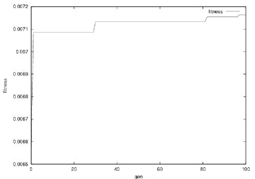
simulator. The population size was of 20 individuals, and we ran the
genetic algorithm for 100 generations.
The initial position was the same for both tasks, with the
crossover and the mutation rates being 0.8 and 0.1 respectively. In
the algorithm, four of the parameters --
in our
simulator. The population size was of 20 individuals, and we ran the
genetic algorithm for 100 generations.
The initial position was the same for both tasks, with the
crossover and the mutation rates being 0.8 and 0.1 respectively. In
the algorithm, four of the parameters -- ![]() ,
, ![]() ,
,
![]() and
and ![]() lie on the positive real axis and hence
we have to choose an upper limit on the real line. This upper limit
is important since a low upper limit value implies that we implicitly
restrict our real valued parameters to that limit, while a high upper
limit value may increase the number of generations for which the
genetic algorithm may have to be run since the initial random
generation will be very disperse.
lie on the positive real axis and hence
we have to choose an upper limit on the real line. This upper limit
is important since a low upper limit value implies that we implicitly
restrict our real valued parameters to that limit, while a high upper
limit value may increase the number of generations for which the
genetic algorithm may have to be run since the initial random
generation will be very disperse. ![]() and
and ![]() are exponents of
numbers less than 1 and hence their large values will not be useful.
Keeping these factors in consideration, the upper limit value has
been fixed to 5 in our simulations.
are exponents of
numbers less than 1 and hence their large values will not be useful.
Keeping these factors in consideration, the upper limit value has
been fixed to 5 in our simulations.
![\includegraphics[width=6cm]{figures/GA/21bestRotsmall}](img265.png)
![\includegraphics[width=6cm]{figures/GA/21averageRotsmall}](img266.png)
![\includegraphics[width=6cm]{figures/GA/21mahalanobisRotsmall}](img267.png)
|
![\includegraphics[width=6cm]{figures/GA/31averageRotsmall}](img268.png)
![\includegraphics[width=6cm]{figures/GA/31mahalanobisRotsmall}](img269.png)
|
The genetic algorithm converges to an optimal solution for each cluster as can be seen in Figures 5.10-5.15. By optimal solution we refer to the best solution the algorithm has found, which may not necessarily be the optimal solution to the navigation task. The optimal values for some of the parameters differ significantly for the two clusters as shown in Table 5.2. The parameters associated to the bidding function of the Risk Manager agent differ the most between the two clusters. This is so because the Risk Manager is very sensitive to the complexity of the task. The more obstacles, the higher the risk of losing sight of landmarks.
In order to check the results obtained for each of the clusters, we
have tested the two parameter sets found by the genetic algorithm on
the two different navigation tasks (going to cluster ![]() and going
to cluster
and going
to cluster ![]() ). We have also tested our original parameter set,
which we set by hand, on the same two navigation tasks. The results
obtained by each set on each of the tasks are shown in Table
5.3. For each task, the mean average success value
(
). We have also tested our original parameter set,
which we set by hand, on the same two navigation tasks. The results
obtained by each set on each of the tasks are shown in Table
5.3. For each task, the mean average success value
(![]() ), average cost (
), average cost (![]() ) and the fitness value
(
) and the fitness value
(![]() ) is computed. As expected, the parameter set found for cluster
) is computed. As expected, the parameter set found for cluster
![]() performs perfectly when going to cluster
performs perfectly when going to cluster ![]() and it only
reaches the targets of cluster
and it only
reaches the targets of cluster ![]() 50% of the time. On the other
hand, the parameter set found for cluster
50% of the time. On the other
hand, the parameter set found for cluster ![]() reaches the targets of
cluster
reaches the targets of
cluster ![]() all the times, while it only reaches the targets of
cluster
all the times, while it only reaches the targets of
cluster ![]() 50% of the time. Finally, the hand-tuned parameter
set reaches 50% of the time for targets in cluster
50% of the time. Finally, the hand-tuned parameter
set reaches 50% of the time for targets in cluster ![]() , and never
reaches the targets of cluster
, and never
reaches the targets of cluster ![]() . Therefore, the evolutionary
approach has improved the global navigation behavior.
. Therefore, the evolutionary
approach has improved the global navigation behavior.
In Figures 5.16 and 5.17 we can see some paths followed by the robot using each of the parameter set on each of the tasks. Successful paths are only shown for those parameter set with a success value of 1. Otherwise, an example of a failing path (marked with a cross at its end) is shown.
© 2003 Dídac Busquets